What is this article about?
Finite element analysis (FEA) is a powerful tool in mechanical engineering. But what happens when it is used incorrectly? Recipients of analysis reports and the engineers who carry them out rely on their calculations to make structures safer, more efficient and more durable. But this is precisely where risks lurk: Inaccurate modeling, incorrect assumptions and incorrect interpretations can lead to catastrophic errors.
How can such errors be avoided? What factors influence the accuracy of simulations? This article highlights the most common stumbling blocks in FEA – and shows how engineers can achieve more precise, reliable results.
A short summary and potential for error
Faulty Finite Element Analysis (FEA) - A Growing Problem in Litigation
In recent years, legal disputes and pre-trial disputes in connection with faulty finite element analyses (FEA) have increased noticeably. As an expert in the analysis of causes of damage, vibration technology and operational stability of machines and their components, I have found that both the lawyers of the disputing parties and the courts are often unaware of the amount of effort that actually goes into such an analysis. Proving that an analysis is faulty is complex, but undoubtedly possible, although usually costly.
Furthermore, simply looking at the usual “colorful analysis pictures” is not enough to provide reliable evidence of a possible analysis error in a legal dispute as a court expert or in a legal dispute as a party expert.
A central problem lies in the increasing popularity and supposed “easy application” of the finite element method (FEM). Modern software solutions suggest that such analyses can be carried out quickly and easily – sometimes even directly in CAD programs. The reality, however, is different: many users do not have the necessary mechanical, numerical and material engineering expertise to correctly interpret the results of a finite element analysis and avoid critical errors.
The result is numerous incorrect analyses in reality. This often goes unnoticed because in many cases “high stresses” are detected, which in practice often leads to over-dimensioned components – an economic problem, but usually not a safety-critical one. However, it always becomes critical when components are to be designed in borderline areas and an incorrect calculation leads to structural failure or even major damage.
Legal disputes in particular show that a careful, methodically correct analysis is essential. The quality of an FEA depends on the professional competence of the user – and this is precisely where an often underestimated risk lies.
What does FEM / Finite Element Method mean?
Part 1 of this article deals with the finite element method and explains some of the basics of FEM. There will be no repetition here.
What does FEA / Finite Element Analysis mean?
Finite Element Analysis (FEA) is a powerful numerical method that enables engineers to simulate and predict the behavior of components and systems within the framework of numerical approximate solutions. It is based on the finite element method (FEM), a mathematical technique that makes complex problems analyzable by breaking them down into smaller, manageable subproblems. While FEM provides the underlying methodology, FEA includes the
practical application process as well as the interpretation of the results generated by the FEM calculations.
The FEM breaks down a complex system into a multitude of small, simple units, the so-called “elements”.
These finite elements are connected to each other at their nodes (Figure 1). Behind this is a complex mathematical system of equations. Once the “boundary conditions” have been defined, the deformations and, from this, the strains and stresses can be determined.

The calculations take into account material properties, geometric configurations and external influences such as loads or temperatures.
Finite element analysis (FEA) serves as a crucial tool in engineering. By using FEA, development times can be shortened, costs reduced and risks minimized. Instead of physical prototypes, virtual models are used that can be tested under a wide range of operating and environmental conditions. This not only reduces the use of resources, but also increases the safety and efficiency of the development process if the method is used correctly.
Important:
The FEA must be carried out technically correctly within the framework of approximate solutions.
Process of FEA / Finite Element Analysis in Mechanical Engineering
The process of finite element analysis usually follows the following pattern:
- Identify and formulate the problem
- Define task
- Preprocessing: Model preparation: The component is broken down into small “finite elements”, e.g. hexahedrons or tetrahedrons, squares or triangles. The mesh fineness has a decisive influence on accuracy and computing time. Parameter definition: Material properties, external loads and boundary conditions are defined and specified. These determine the behavior of the model under load.
- Analysis: The FEM software solves a complex system of equations that describes all interactions between nodes and elements. Iterative methods are used for nonlinear problems.
- Postprocessing: Results such as stress distributions, deformations or temperature fields are evaluated graphically and numerically. Critical areas are analyzed and plausibility checked.
Finite Element Analysis (FEA) faulty / error potentials
Despite its wide acceptance and performance, the application of finite element analysis (FEA) contains potential sources of error that can lead to inaccurate results or misinterpretations. These errors often result from assumptions, simplifications or improper handling of the method. The most important potential errors when applying FEA are listed below:
Inaccurate modeling
The influence of the elements was discussed briefly in section 3.2 in part 1 .
Which model is correct?
There is the following definition:
Common problems are:
Geometric simplifications: To reduce calculation time, simplifications are often made to the model geometry. This can lead to important details such as small radii, holes or specific geometries that affect local stresses not being taken into account.
Incorrect material properties: Inaccurate or insufficiently tested material data can lead to erroneous results, especially for anisotropic, nonlinear or time-dependent materials.
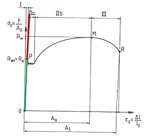
A “classic” case of incorrect analyses is that the calculation continues linearly along the green Hooke’s line (red in Figure 3) even beyond the yield point. The hardening is not taken into account and the result is
correct in terms of mathematics, but completely wrong in terms of reality,
because the material properties “above” the yield point no longer behave linearly (green area) (Figure 3).
Unrealistic boundary and load conditions: Assumptions about the actual loads, supports or environmental conditions are often inaccurate. Incorrect assumption or knowledge of the loads can cause significant deviations from reality.

Three
necessary criteria
are important for the assessment (Figure 4):
- External loads (forces, pressures, temperatures, etc.) act on the component. This is marked with the number 1 in Figure 4.
- The external load results in stresses in the structure. These must be known or determined. This is marked with the number 2 in Figure 4.
- If these internal stresses are known, they can be compared with the mechanical properties of the material used. If the corresponding stresses occurring in the material are greater than or equal to the mechanical properties of the material used, the component can fail due to different types of failure depending on the type of load (static, dynamic).
What is essential, however, is that the external load is known and, above all, what results from it in the component.
Numerical errors
When applying the finite element method, one should never forget that the result of a finite element analysis is a numerical procedure.
If a result can be generated, then the mathematics is certainly “correct”. If this were not the case, no result would be obtained. The crucial question, however, is whether the “result” is plausible or can be plausible. However, if the model is faulty, then the mathematics can “calculate correctly”. However, the result is then
mathematically correct but still wrong in reality.
It is therefore the great art to
To know or be able to estimate the error potential in a finite element analysis (FEA).
Discretization: A model mesh that is too coarse (too few or too large elements) may not correctly represent important local effects, such as stress peaks or deformation details. On the other hand, elements that are too small lead to long computing times without always providing a significant gain in accuracy.
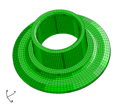
Figure 5 shows an analysis model made up of hexahedral elements. These are of “high quality”. However, they can only be used for rotationally symmetric solid bodies or regular bodies such as cuboids.
However, the reality of technical problems deviates from these ideal geometries.
This alone leads to a decrease in accuracy compared to the quality of the results of hexahedral elements. This will be discussed later in this article.
Element types: Choosing inappropriate finite element types (e.g. linear instead of quadratic elements) can have a significant impact on accuracy.
Rounding and approximation errors: Numerical calculations are susceptible to rounding errors, especially in complex models with many iterations. These errors can accumulate and distort the results.
Incorrect interpretation of the results
Over-reliance on simulation results: FEA results are based on assumptions and simplifications and are
always approximate solutions.
Uncritical acceptance of the results without validation through physical tests or experience can lead to wrong decisions.
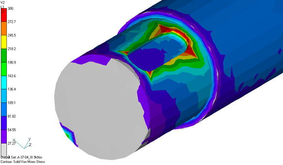
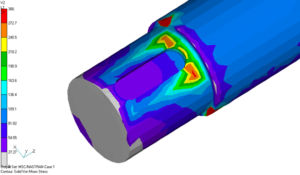
Figure 6 and Figure 7 show an analysis with the same external load but slightly different support conditions. Clearly, one can see significant changes in the determined stresses at the keyway.
The question arises: which analysis better reflects reality?
Does the layman immediately recognize which solution is likely to be wrong and which is closer to reality? This is precisely the central problem with analyses using the finite element method. Anyone who only sees the color “red” and “searches” at the same time is susceptible to incorrect results, incorrect interpretations and possibly also to “problems” that are not problems at all in reality.
Neglect of uncertainties: There are numerous real uncertainties that are not and cannot be taken into account in an analysis. For example, the analysis always assumes a stress-free state. This is a fallacy, because
Often, even in the unloaded state, so-called residual stresses are already present in the structure.
The extent of these is often unknown. There are also other influences, such as
- manufacturing tolerances,
- material variations,
- load changes,
- manufacturing,
- transformation,
- component size,
- etc.,
which are often not included in the analysis, which can distort reality.
Overlooking local effects: Looking at the overall results without analyzing critical areas such as edges, holes or transitions can lead to load peaks being overlooked or misinterpreted.
user error
In my experience, this error is the most common error in finite element analysis.
A large number of calculations are carried out on the analysis market. In my experience, only a minority of engineers are aware of the mechanics and numerics used in the background of the software in the finite element method. This is precisely the biggest problem: for over two decades, providers have repeatedly communicated on the market that any engineer can work with the software. In the end, this may even be true. However, anyone who does not know what is being calculated and where the problems arise due to the numerics and the approximate solutions is not at all in a position to correctly classify the “produced results” of an analysis.
Lack of expertise: Using FEA software usually requires in-depth knowledge of mechanics, materials science and numerics. Inexperienced users can make mistakes when creating models or evaluating results.
Automated processes without verification: Modern FEA software often offers automated processes, e.g. for meshing or solution control. Blind trust in these automations can be problematic if the underlying assumptions are not verified or, in most cases, are not even known in detail to the operators of the “black box”.
computing time and resources
It is a well-known phrase:
Time is money.
This also applies to the finite element method and a finite element analysis (FEA).
If you want to create a high-quality FE mesh as part of the modeling process and thus the basis for a meaningful finite element analysis, serious modeling is complex and can rarely be created automatically using a preprocessor. It requires manual work and the use of know-how by the calculation engineer, who ideally is also very experienced. The size and quality of the calculation model also increases the time required to carry out the analysis. This also means effort and costs. Due to ever faster computers, hardware has become cheaper over the years. Nevertheless, this is a cost factor that should not be underestimated.
In reality, structural areas that are difficult to model are often simplified in the analysis. This saves time for modeling and analysis effort. This can be done if you are a very experienced calculation engineer and have a “good feeling” for the expected analysis result. This, in turn, requires years of calculation experience.
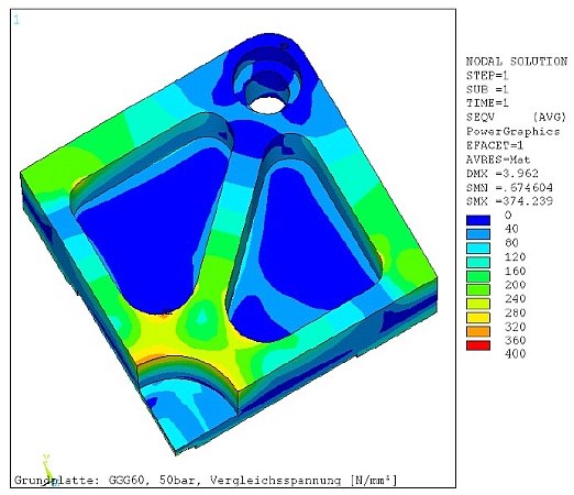
Figure 8 shows an analysis result with a symmetrical model, where the symmetry was used to reduce the model and thus the analysis effort. This approach can be used for symmetrical loading and component symmetry. However, in the model in Figure 8, it was also “forgotten” to model an important structural area in detail during modeling because the calculation engineer carrying out the work was not experienced but possibly wanted to save time. The result of this model simplification can be seen in Figure 1.
Figure 1 shows a structure that had failed in reality and Figure 9 shows the pictorial representation of the principal stresses in the affected cross-section determined using the Finite Element Method (FEM).

When comparing Figure 1 and Figure 9, it is immediately apparent that, with correct modelling, significant stress increases were also identified in the analysis in the fractured area of the structure. With correct application of the FEM, known external loads, expert modelling followed by analysis and evaluation, the FEM allows such problems to be identified in advance.

In the analysis shown in Figure 8, the critical area according to Figure 9 or Figure 1 was not even modeled. In this respect, the problem could not be identified at all in the context of the finite element analysis.
The consequence was damage that caused a machine that had just been launched onto the market to fail after a short period of operation in the USA, Europe, Asia and Australia. A worldwide product recall was the result.
In short, this means for this type of error possibilities:
Shortcuts due to time pressure: In order to save computing time, assumptions or simplifications are often made that affect accuracy.
Hardware limitations: Complex models require high computing power. Limitations in available hardware can limit model complexity or analysis accuracy.
Insufficient validation
Validation is generally desirable and recommended. Of course, the purpose of an analysis using the finite element method is to minimize or, if possible, completely avoid complex experiments and tests.
Therefore, in reality, validations are only carried out where a high number of components/machines are produced or where a failure has had major consequences. The leading examples of validations and checks through further tests are
- the automotive industry and
- the aviation industry and
- the space industry.
In other areas of mechanical engineering, for cost reasons, no or very few experimental tests are usually carried out to verify the simulation results. This is why this error possibility is of somewhat minor importance in reality.
Briefly and succinctly, this error potential is listed:
Lack of comparative tests: Simulation results should ideally be validated by experimental tests or analytical calculations. Without this validation, undetected modeling errors can lead to incorrect conclusions.
Ignored limit cases: Tests of extreme situations, such as maximum loads or critical operating conditions, are often neglected, although they are essential to assess the limits of model accuracy.
Nonlinear Effects and Complex Physics
Figure 10 shows a typical stress-strain diagram for ductile steel. The material behavior is linear only in the region of the so-called Hooke’s line.
If the determined stresses from external loading in the stressed cross-section are within this range of linearity, the resulting strains return to the undeformed initial state when the load is removed. However, if the yield strength of the material is exceeded, plastic strains remain when the load is removed. The material is then permanently deformed and damaged.
However, if one continues to calculate linearly beyond the yield point, the mathematics may be “correct”, but it no longer has anything to do with reality because the material properties no longer behave linearly above the yield point.
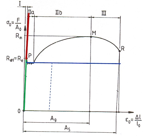
Nonlinear analyses are always more complex and usually take more time. Of course, in reality, when analyzing most materials, there is no stress-strain diagram available from which the hardening after the yield point is exceeded can be realistically depicted. So if in reality you calculate with hardening and thus nonlinearly, the calculation is “horizontal”, so to speak. After the yield point is exceeded in the linear range, marked green in Figure 10, the calculation continues elastic-ideal-plastic. This is marked with the blue horizontal in Figure 10. It is a conservative assumption in calculations, if nonlinear calculations are used at all. This means that you are on the safe side in the analysis, but under unrealistic assumptions. However, it is the simplest way to take a nonlinear approach to hardening into account.
Briefly and succinctly, this error potential is listed:
Neglecting nonlinear phenomena: In practice, many problems are nonlinear (e.g. plastic material behavior, contact problems or large deformations). A linear finite element analysis cannot correctly represent such effects.
Multiphysical interactions: When several physical effects act simultaneously, neglecting one aspect can lead to inaccurate results.
influence of the elements
The structure to be assessed is divided into a finite number of small and simple geometric elements (“finite elements”) that are connected to each other at their nodes (Figure 11). This is based on a complex mathematical system of equations. Once “boundary conditions” have been defined, the deformations and, from this, the strains and stresses can be determined.
These finite elements are connected to each other at the so-called nodes (Figure 12). The decisive, continuously changing quantities of the problem are represented by their values at the nodes. Continuous functions are replaced by a system of a finite number of node parameters. The solution of the individual parts ultimately results in the approximate solution for the idealized overall structure.

For different problems, there are different elements, for whose node displacement mathematical approach functions are defined that influence the result. Anyone who is not familiar with this as a “software user” cannot even
not objective
evaluate.
A distinction is made between one-dimensional, two-dimensional and three-dimensional elements.
One-dimensional elements are beams and rods, which can often only be used for very simplified questions.

“ Thin ” structures are represented with two-dimensional shell elements. We speak of “ structurally thin ” when one dimension is much smaller than the other two dimensions. The hood of a car, for example, is a classic structurally “thin” structure.
Structures that must be captured using volume elements include bearing blocks, rollers, engine housings, etc.
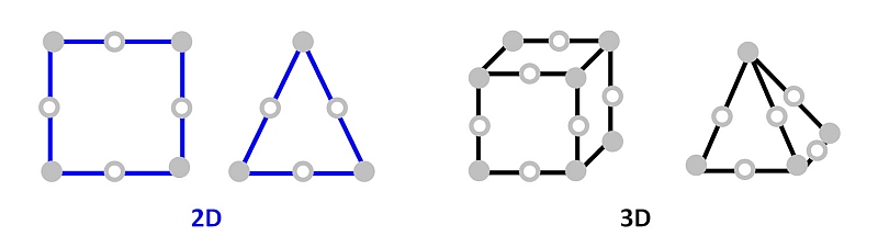
Figure 12 shows common elements for thin structures (2D) and for volumes (3D). All elements in Figure 12 are linear elements.
There are also elements with higher approaches (Figure 13).
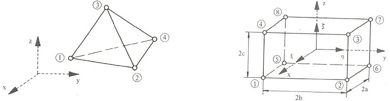
The linear tetrahedral element has 4 nodes. The linear hexahedral element has 8 nodes. For each node, displacements in the underlying Cartesian coordinate system are generally established.
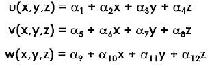
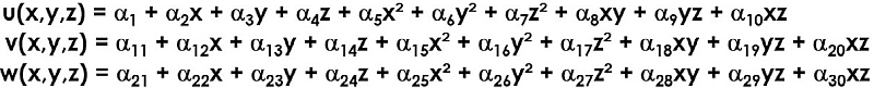
Figure 15 shows the general displacement approaches taking into account the 12 so-called generalized coordinates required for this. It can be seen that the proportional displacements in the direction of the respective coordinates can only be taken into account with a linear approach, since the number of generalized coordinates per displacement component results from the number of nodes.
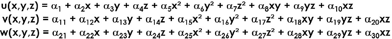
Figure 16 shows the general displacement approaches taking into account the 24 so-called generalized coordinates required for this. This number arises because the linear hexahedral element has eight nodes, for which three displacement components under load must be determined in the Cartesian coordinate system. When comparing the equations to be solved for a single element, it is clear to any layperson that the approach according to Figure 16 contains significantly more terms. Quadratic mixed terms are added and in the last component there is also a product of all components, i.e. to the third power. What can be derived directly from this:
Solutions with hexahedral elements are always within the scope of the approximate solutions due to the approaches
more precisely
than with tetrahedral elements. The fatal thing about volume structures in reality, however, is that the possible uses of hexahedral elements are limited because real structures do not represent “ideal” bodies, such as cuboids or rotationally symmetrical structures.
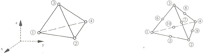
On the right in Figure 17 you can see that another node is included between two end points and thus the nodes of the tetrahedral element. This increases the number of nodes from 4 nodes to 10 nodes.
When comparing Figure 18 and Figure 15 of the equations to be solved for a single element, one can see that quadratic and mixed quadratic terms are now added to the tetrahedral elements with an increased number of nodes.
From this, even a layman can clearly see:
- the analysis effort is (significantly) increased,
- the result is more accurate within the framework of numerical approximate solutions.
If you now take into account the higher number of nodes in the hexahedral element, the system of equations to be solved increases considerably. This costs computing time, memory and tends to lead to files for the results exploding.
This example is intended to illustrate how the choice of elements influences the quality of the result, but also the computing time and thus the costs (“time is money”).
As a calculation engineer, you must therefore know very well what you are doing and, in case of doubt, choose an increased discretization of the structure in structural areas where it is necessary.
However, if you are just a software user and use ready-made meshes provided by a simple CAD program and blindly “believe” the result, this may work in many cases. But if it is important and accuracy is literally important,
An experienced calculation engineer with appropriate knowledge of the theory, its application and the software is required.
quality requirements for elements
There are also quality requirements for elements in a FEM calculation.
It is quite clear that the elements used cannot be “ideal” squares or triangles in the two-dimensional case. In the same way, the elements used cannot be ideal tetrahedral elements or hexahedral elements in volumes that are mapped across an entire structure. This means that the elements of a mesh are almost predominantly distorted in some form. The reader of an analysis report after a finite element analysis (FEA) has been carried out does not learn anything about this.
In many programs, the “operator” does not even have the option to intervene in the network quality. Of course, the quality of the elements also determines the result and its quality.
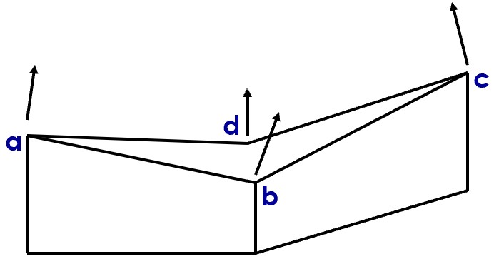
Figure 19 shows an example of a hexahedron element in which the nodes do not lie in one plane. Ideally, in a linear hexahedron, four nodes of the six different planes lie in exactly the same plane. However, this is just theory. This is almost never the case in real structures. The consequence of such effects is that the quality of the result of a “deformed” element is reduced. Experts then know what to do and how to interpret the analysis result.
Other quality characteristics include:
- skew,
- aspect ratio,
- Rejuvenation.
Networking and its influence
With a finer discretization (mesh fineness), the approximate solution theoretically converges to the (exact) solution, which, however, is based (only) on analytical approaches, which also represent approximate solutions.

However, a finer mesh with lower-quality tetrahedral elements does not provide “more accurate” results than a coarser mesh with higher-quality elements.
The precise knowledge of the elements and, in addition, a technically high-quality discretization (networking) provide the necessary basis for an analysis result with good information quality.

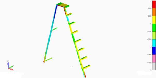
In principle, it is possible to visualize stresses and displacements in a structure while taking into account bearing boundary conditions and external loads. This is shown in Figure 21 for the model in Figure 20. It should never be forgotten that these are approximate solutions.
Important:
Often an optimal element division can only be achieved through appropriate experience!
It is precisely this fact that creates great potential for error when users work with this finite element method without having detailed knowledge of the underlying technical mechanics, mathematics, physics and materials science.
Conclusion
In order to minimize the potential for errors when applying finite element analysis, a
Careful planning and validation of the model is essential.
Engineers should always critically question the assumptions and results, use suitable validation methods and take into account the limitations of finite element analysis. Only through a solid understanding of the underlying theory and conscientious implementation can reliable and meaningful results be achieved.
Structural Mechanics - Some Basics
Tensions
A stress is an auxiliary quantity which, in a one-dimensional case, results quite simply from the quotient between the acting force F and the underlying area A:

If the maximum permissible stress is exceeded, the structure will be damaged. A distinction is made between static and dynamic stress. In the dynamic case, only lower maximum stress values or stress amplitudes can be tolerated.
material hardening
steels
In the tensile test, steels exhibit a stress-strain diagram, which can in principle be derived from the general example in Figure 10.
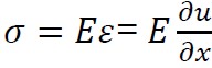
In the linear-elastic region I there is a linear relationship between stress and strain (Hooke’s law, section 6.7, Figure 10) in the form:
The elastic modulus E is a material constant.
yield strength and 0.2% yield strength
The yield strength Re characterizes the end of the linear-elastic material state and thus describes the failure by flow, i.e. by the onset of plastic deformation, see Figure 10.
In many structural steels, a pronounced yield region with an elongation of 1-3% follows (region IIa in Figure 10).
tensile strength
In area IIb the increase is non-linear. The material flows. It deforms plastically.
In area III, the test bar begins to constrict at the weakest point. Eventually, a crack occurs. This determines the tensile strength .
strength hypotheses
In reality, material properties are determined in the laboratory on smooth samples under a defined stress state. Most of the time, these are uniaxial stresses in tensile tests or bending tests.
Since a component is usually subject to any multiaxial stress state during operation, a comparison between component stress and the material properties is not easily possible.
Therefore, transfer functions are required that convert the multiaxial stress state into an equivalent uniaxial stress state. These transfer functions are the strength hypotheses with which a so-called equivalent stress is calculated.
normal stress hypothesis
The normal stress hypothesis applies to
brittle material behavior .
According to the normal stress hypothesis, failure by separation fracture occurs under static loading when the maximum normal stress reaches the separation strength of the material.
Brittle fracture occurs perpendicular to the largest principal stress.
shear stress hypothesis
The shear stress hypothesis assesses failure by yielding and, under certain conditions, by shear fracture. According to the shear stress hypothesis,
The largest shear stresses occurring in the body are decisive for failure.
shape-change hypothesis (flow condition according to von Mises)
The shape change hypothesis is originally derived from the yield condition according to von Mises , according to which the flow in an isotropic body must be independent of the position of the coordinate system (invariant) and the hydrostatic stress state makes no contribution to the flow.
According to the shape change hypothesis,
Failure by yielding occurs when the equivalent stress has reached the value of the yield strength Re.
Comparison of shear stress hypothesis / shape change hypothesis
Both hypotheses describe the failure
ductile (deformable) materials
by flowing.
Thus, in principle, it is possible to choose one or the other hypothesis for these materials. However, technical regulations often prescribe the use of one of the two hypotheses.
"Classics" for faulty finite element analysis (FEA)
Laypeople and unfortunately also many engineers or designers who only use the software as a “black box” cannot correctly evaluate analysis errors or the results of the finite element analysis (FEA). Some “classics” for faulty finite element analyses (FEA) are listed in the subsections. There are many more examples than those listed here in the subsections.
External loading of a structure (“1” in Figure 4) causes corresponding stresses in the interior (“2” in Figure 4). The expert also differentiates between different stresses. These must be evaluated using the “correct” strength hypothesis.
Analysis along Hooke's line
If these stresses exceed the yield strength of the material, permanent deformations (plastic deformations) occur when the load is removed. Dynamic stress results in much more complicated effects. These are not discussed in this paper due to the scope of the paper.
Calculations with linear material behavior, i.e. with linear material law, immediately become incorrect if the determined stresses exceed the yield strength of the material used (Figure 10).
The verification is relatively simple if the material is known from the analysis results provided:
Is the legend scaled regarding the yield strength?
If this is the case, one can assume, at least in a first step, that the engineer carrying out the work knows that only stress results up to the yield strength of the material make technical sense in a linear analysis.
However, it is technical nonsense to extrapolate and subtract arbitrarily along the Hooke’s line in order to “evaluate” structural modifications – often in reality. This has already been explained in section 6.7 and in Figure 10 in this article.
Strength hypothesis and component material do not match
It is almost “usual” that almost exclusively Von Mises equivalent stresses are evaluated.
For analyses of cast iron structures, the Von Mises equivalent stresses are often evaluated on the analysis market. In such a case, the engineer carrying out the analysis has “forgotten” that cast iron is a brittle material and that the principal stresses are crucial for failure.
Anyone who is presented with an analysis result for a cast component and realises that Von Mises equivalent stresses were used for the assessment knows immediately that the
The calculator simply did not really know what he was doing and was just a user of the “black box”.
The fatal thing is that many clients have no knowledge of finite element analysis and
seem to blindly trust the analysis reports with colorful pictures.
It becomes problematic when structures fail in reality.
Dynamic loading and evaluation "static"
Very often, when reviewing analyses in the event of a damage event, I find that the analysis and evaluation of ductile materials was actually correctly based on the yield strength.
However, different failure criteria apply if the loading is dynamic.
In such a case, the analysis may be mathematically “correct” within the framework of the numerical approximate solutions. However, if the type of stress is not static, the evaluation must not be carried out according to static criteria. This is a very common error in reality and always an indication that the person doing the calculation is merely a software user and unfortunately does not understand in detail what he is actually analyzing and executing.
Wöhler diagram
Figure 22 shows a purely schematic Wöhler diagram. These diagrams are used to describe the fatigue strength behavior of components as a function of the number of fatigue cycles. The number of cycles is plotted logarithmically.
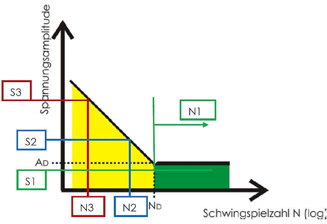
There are essentially two areas:
- an inclined line and
- a horizontal.
If this diagram is based on a Cartesian coordinate system, the stresses are taken into account on the ordinate and the vibration cycles on the abscissa.
For detailed explanations, please refer to section 3.2.1 in the article “ Destruction of evidence in the legal dispute ‘Vibration resonance ’ in machines ”.
Important:
The stresses occurring in a cross-section to be assessed as a result of vibration loading must be less than or equal to the value for the fatigue strength (A D in Figure 22).
The yield strength Re is therefore irrelevant for the assessment in a finite element analysis (FEA) under dynamic loading, even for ductile materials.
The base plate of an industrial press was chosen as an example. This simple structure can be represented using hexahedral elements as well as tetrahedral elements.
The load acts centrally on a circular surface. Only a quarter model was considered. With symmetrical loads and geometric symmetry, identical results are achieved with reduced models and thus less analysis effort.
Follow-up calculation: Stresses are always less accurate than displacements
In the static case, the software solves a system of equations of the form
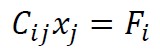
The displacement vector x_j contains the cone displacements of the elements. C_ij is the stiffness matrix. It depends on the number of nodes and the generalized coordinates of the displacement approaches, is “unimaginably large” and must be inverted to solve the problem. F_i is the load vector.
In order to determine a stress, it is important to know the strain. Strains are determined from the derivatives of the displacements, i.e. in the exemplary one-dimensional case from
Since differentiation is not possible in the context of follow-up calculations with numerical programs, the difference quotients are formed.
As a consequence, stresses from the follow-up calculation are always less accurate than the displacements.
boundary conditions
In the area of
- load introductions,
- storage boundary conditions,
- discontinuous structural transitions,
- Corners and edges in the model, but also
- for elements with degenerate (“corrupt”) geometry or, for example,
- also elements whose nodes are not exactly connected to each other,
“High” voltages are often identified. However, these are
not given
and one
consequence of numerics .
Figure 23 shows a trivial mechanical equivalent model. A bar with the cross-section and the modulus of elasticity is fixed at one end. Displacements are not possible in the area of the support. The other end is pulled with a force.
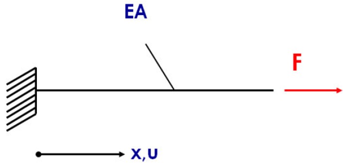
The stress is determined numerically in a follow-up calculation according to equation 2 from the difference quotients of state 1 (“unloaded”) and state 2 (“under load”).
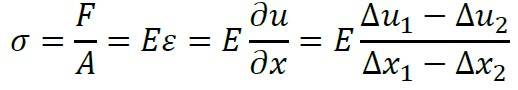
If no change can occur in the clamping state either under load or without load, the denominator will be identically zero, i.e.
The mathematically correct answer is:
In mathematical terms, this means:
and thus “high tensions”. This is
mathematically correctly determined;
only
technically it is completely wrong!
Anyone who does not know this and is not aware of what the software really does as a result of the numerics – which is unavoidable, mind you – produces technically incorrect results and unfortunately often believes them.
Visually, this can be seen in the results through areas of significant voltage increases or through “color crumbs”. All of these results are
technical nonsense, result from the numerics underlying the analysis program and can not or only partially be avoided.
Unfortunately, many “software operators” are not aware of this.
Example of the influence of tetrahedral elements and hexahedral elements in modeling
The base plate of an industrial press was chosen as an example. This simple structure can be represented using hexahedral elements as well as tetrahedral elements.
The load acts centrally on a circular surface. Only a quarter model was considered. With symmetrical loads and geometric symmetry, identical results are achieved with reduced models and thus less analysis effort.

Figure 24 shows the comparison of the determined displacements for one and the same structure under identical loading for tetrahedral elements (3D “right” in Figure 12) and for the hexahedral elements (3D “left” in Figure 12) with identical scaling of the results. The difference in the determined displacements is 22.9%. The structure is simply calculated to be “stiffer” using the tetrahedral elements.

Figure 25 shows the same comparison, but for the determined Von Mises equivalent stresses at identical scaling.
As expected, the differences in voltages are larger.
The reason for this is the follow-up invoice.
Hexahedral elements calculate larger displacements (22.9%) and also higher stresses (25.0%) under otherwise identical conditions.
These are crucial differences.
This must be kept in mind when conducting analyses and/or receiving results.
Some error possibilities as (negative) multipliers
In the previous sections, some possible errors were presented and discussed. Of course, only the most common errors in my experience were listed. There are numerous ways to introduce errors into a calculation using the finite element method and thus carry out the analysis incorrectly.
The following aspects are essential:
- Only numerical approximate solutions are determined.
- The approach functions refer to analytical model approaches of (linear) engineering mechanics.
- The task influences the elements to be applied.
- The element type influences the quality of the results.
- Network quality and network fineness are reflected in the result of the analysis.
- Linear calculation across Hooke’s line is technically incorrect.
- The correct load assumptions are essential for the result. If the load assumptions are incorrect, the end result may not be correct anyway.
- Stress results are always less accurate than the determined displacements.
- Results at storage boundary conditions are never correct.
These potential errors influence the final result in multiple ways and are therefore negative multipliers. And that is precisely why you have to be very critical when confronted with analysis results.
What is strange, however, is that errors in the analyses lead in most cases to “high” stresses. If something like this is determined incorrectly, measures are taken to reduce the “high” stresses. If everything goes “well”, you end up with an oversized structure. In reality, nothing breaks, despite the incorrect result.
However, things become critical when precise dimensioning becomes necessary.
This often leads to failure in reality. When computational analyses are increasingly presented in legal disputes, the results are often “calculated well”. It is extremely difficult to check the plausibility of such analyses if the analysis data is not made available. However, as an expert, you can then use the result plots to identify whether there are any indications of errors.
But only experts can recognize this. There are few of them and in the field of expert witnesses there are perhaps only a handful.
basic requirements
An engineering degree with in-depth knowledge of mathematics, technical mechanics and physics is necessary. In my opinion, the focus should be on technical mechanics, strength of materials and vibration technology. It is also helpful and self-evident,
Lectures in the Finite Element Method
visited and understood. This in turn requires
sound knowledge of technical mechanics
Unfortunately, technical mechanics is a subject that is not very popular among students because it is considered “difficult”.
If you meet the above requirements, you also need
practical experience.
Results must always be critically questioned, ideally discussed with other true experts and research carried out. The exchange of information is essential.
The technical skills of a calculation engineer include
- modeling,
- the analysis with the evaluation,
- the documentation,
- presentation and also
- critical discussion of the results.
This involves gathering experience that, over the years, leads to an ever-increasing wealth of experience, so that at the end of the day, you actually become an expert . Calculation engineers are engineers who require high technical and personal requirements. Unfortunately, this is often not appreciated, because it is not usually the technical specialist who makes a career in industry.
Conclusion
Finite element analysis ( FEA ) is an indispensable tool in mechanical engineering and many engineering disciplines. It enables the precise simulation of mechanical loads and helps to make development processes more efficient, reduce costs and minimize safety risks.
However, the application of finite element analysis
considerable potential for error.
Inaccuracies in modeling, inadequate discretization, incorrect boundary conditions and a lack of specialist knowledge can lead to unrealistic results. This becomes particularly critical when components are dimensioned in borderline areas or safety proofs have to be provided. Increasing automation and the integration of FEM in CAD software increase the risk that calculations are carried out without a full understanding of the underlying mechanical and numerical principles.
To ensure the quality of finite element analyses, in-depth knowledge of technical mechanics, materials science and mathematics as well as numerics is required. In addition, simulation results must always be critically questioned and, if possible, validated by experimental tests or alternative calculation methods.
Litigation has increased over allegations of faulty finite element analysis (FEA).
Especially in legal disputes, it becomes clear that an incorrect finite element analysis can have serious economic and safety-related consequences. Proving such errors is complex, but possible with the appropriate expertise, but is usually costly. This underlines the importance of
qualified calculation engineers
and
careful modeling.
Ultimately, finite element analysis remains a powerful but demanding tool that can only be used
proper use
can develop its full potential.
Recommendation:
Only have a finite element analysis (FEA) carried out by professionals. If you have damage caused by an incorrect analysis, hire an expert experienced in FEM/FEA to carry out the investigation.